= Artificial Intelligence ||
 = Low Level Programming & Systems ||
 = Machine Learning ||
 = Data Structures and Algorithms
= Artificial Intelligence ||
= Low Level Programming & Systems ||
= Machine Learning ||
= Data Structures and Algorithms
This project is probably my most impressive to date, and was a blast to work on! My position as a Founding Officer with NeuroTechSC, as well as Curriculum Lead, allowed me to see all the facets of our Synthetic Telepathy project and
watch it all come together. By the time of submission, we were able to reach 85-90% accuracy on yes/no questions + a small corpus of words, no small feat! As part of the officer team I helped design the project architecture, put together
the teams, and administrated all while giving programming/neuroscience advice to any members of any of the teams. It was a massive commitment, but it paid off.
In addition to more grants and extra funding, I learned a lot about the current state of the BCI (Brain-Computer Interface)
space, as well as N400 ERP-related neuroscience. My leadership skills also certainly improved over the course of the project, and I obtained valuable experience in resolving interpersonal conflict. Check out the team-specific writeup below as well as the links on the left!
NeuroTechSC has successfully submitted their project into their first NueroTechX competition! NeuroTechSC submitted their project, Boole-pathy, into the open challenge. You can find the submission video here. The following is an overall timeline of each team and their progression throughout the project.
Hardware Team
The hardware team was in charge of making the physical device wearable and to take recordings, providing the raw data for the data team.
In the beginning, various members of the team were unfamiliar with the CAD software (Fusion 360). The use of this software was optimal for the online collaborative environment brought on by the Covid-19 pandemic. After team members familiarized themselves with the CAD software, they began to brainstorm possible designs to enclose the OpenBCI board, its battery pack, and the electrodes that attach to the user’s face. In the early stages of design it was thought that a headset would enclose all the components mentioned above. However, this proved to be too much weight and the final design has the electrodes housed on the headset while the rest of the components are kept on the user’s bicep.
There were several challenges the Hardware team had to overcome that were mainly caused by the pandemic. One difficulty was having multiple iterations of the board enclosure made. This had all the hardware components remain with one team member until the final 3D printed product was made. It had to remain with the person who had access to the 3D printer so corrections to the design could be immediately made. This wouldn't have been an issue regularly but team members were not located in each other's immediate vicinity.
As for the gathering of data, the Cyton board along with the electrodes were interchanged amongst team members who followed these instructions to complete recordings. This was until the components had to spend some time with the 3D printer to run through multiple iterations. Finally, it was handed off to the final team member that demonstrated the headset’s use in the presentation. They put on the finishing touches like attaching copper wire to the headset which was used to stabilize and guide the electrodes with the use of shrinkwrap. This brings us to the final product submitted to the NeuroTechX competition.
Data Team
The data team in NeuroTechSC oversaw the pipeline of the project. They were taking in the data from the hardware component, analyze and filter the data, then sending the data to the machine learning team. Their work was very essential to the outcome of how functional the project turned out to be. The data team first began creating the pipeline from the hardware team using BrainFlow, an application program interface that allows you to acquire data from biosensors, parse it, and then analyze it. It is a powerful tool that allows you to receive data from various boards without having to change your code. The data team decided to write their code in the Python programming language.
The team focused on creating a pipeline that received Electromyography (EMG) data. Because they finished creating the basic pipeline early on in the project, they still had not received any data from the hardware. Therefore, in order to get practice, the team members trained with this model. They began to get practice using different forms of data processing, like normalization, Independent Component Analysis (ICA), and using filters like the Butterworth Filter. Once they began working with actual data, they encountered several problems, the main one being that most of the data was being removed when processed. The team narrowed the problem’s cause to come from the form of data analysis, specifically the IPA they were using. After adjusting and testing, they found that using solely filter, IPA, and standardization yielded better results, removing normalization from their pipeline. With this improved pipeline, the team was able to reach an accuracy of 85 percent.
For the remainder of the project, the data team collected new incoming data from the hardware, each data containing new recordings from different individuals. The pipeline accuracy varied from each recording, so the team tweaked and fixed the pipeline. By the end of the project, the data team was able to reach an accuracy of around 85 percent for all data.
Machine Learning
The machine learning team was in charge of analyzing the data sets and predicting if the data given was a ‘yes’ or ‘no’. In the beginning, the team had to choose between using 1-dimensional or 2-dimensional convolution data. Even though 2-dimensional data shows a lot more, is sometimes less accurate, harder to implement, and less efficient so they chose to use 1D. Next, they split into two teams, one working on the convolutional neural network(CNN) model and the other working on the recurrent neural network(RNN) model. Eventually, the team ended up basing their model on the EEGNet paper which is a CNN for EEG-based brain-computer interfaces. This model yielded better results and after training it for a while, they were able to predict with 85-90% accuracy.
UI
The User Interface (UI) team was in charge of creating a full-stack web interface for the project. The team decided on using Reach, an open-source JavaScript, to create the interface. For the backend development, the team decided to use Flask, which is written in Python. While frontend development is used for web interfaces, backend development is the hidden software that a user does not see but essential to creating a website. For this project, the UI team was required to display a yes/no question, create a countdown, then display detected answer onto the interface.
The UI team began by creating a boilerplate code, which is code that can be reused with little change. This code displayed random questions and an answer, which was used as a placeholder until they received actual data from the machine learning team. As they waited for data, the team members began to familiarize themselves with web interface techniques, like technology stacks which are used to build and run web applications. The team also worked with the data team and its pipeline to create the interface. The team concurrently worked on integrating the frontend interface with the backend as well as creating the 2-second countdown.
After creating their first version of the interface, they were able to successfully connect to the machine learning data and display the prediction onto the web interface. Their next steps were to connect to the hardware and display the port number. The team struggled a bit with this but eventually were able to successfully connect. The UI team then focused on finishing touches to the web interface for the final submission.
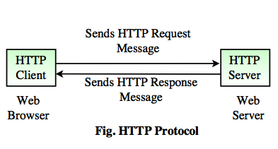
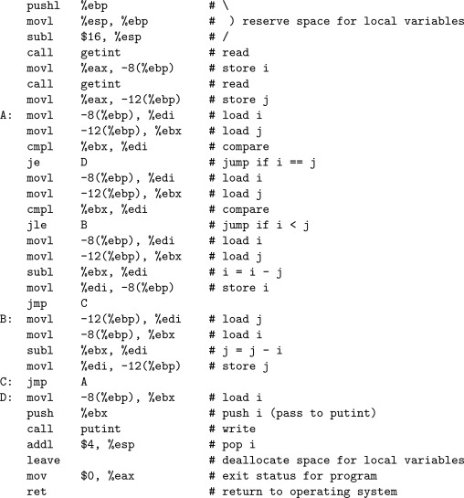
This project was incredibly difficult! Writing a load-balanced multi-threaded server in C is no joke, so beware anyone who tries the same! Implementing GET, HEAD, PUT, and more HTTP requests takes a lot of work in C. My main handled argument handling and thread creation, while my healthcheck module balanced the load by multiplexing requests over a variety of servers. Each server in the array also has multiple threads, which need to be synchronized with synchronization primitives such as mutexes, condition variables, or semaphores. Any given server also has a random chance to go dark completely, in which case my program gathers the available data from storage and redistributes load across the previous servers. This was done with standard libraries and POSIX.
Dispatcher:
The dispatcher thread takes the requisite arguments from main and starts to listen at the correct port, accepting
connections in a loop forever. Once a connection is accepted, it is placed on a queue that the worker threads have access to.
Additionally, the dispatcher is in charge of sending periodic health checks. It shares a condition variable with the healthchecker
that it triggers every R requests.
Healthchecker:
My healthchecker thread utilizes a complicated timeval struct in order to tell time, and uses the condition variable
from dispatcher in order to block itself. It triggers every R requests or 4 seconds.
When it sends a healthcheck to the server array it picks the best server and stores that in a server struct that carries information about all of the servers.
This server struct is shared by the workers, and they use it to prioritize which server they should give work to.
Workers:
These workers are triggered by dispatch whenever an item is placed in the queue. They dequeue this object, and tell the client port.
They then reference the server struct to gather the best server for sending the request to.
After a server is selected and the job is underway, they continually transfer data between the server and the client until one of them closes the connection.
When that job is finished the thread transfers all remaining data to the other side of the connection and goes back to sleep, waiting on the condition variable in dispatch to signal it.
Code and further explanation are available upon request.
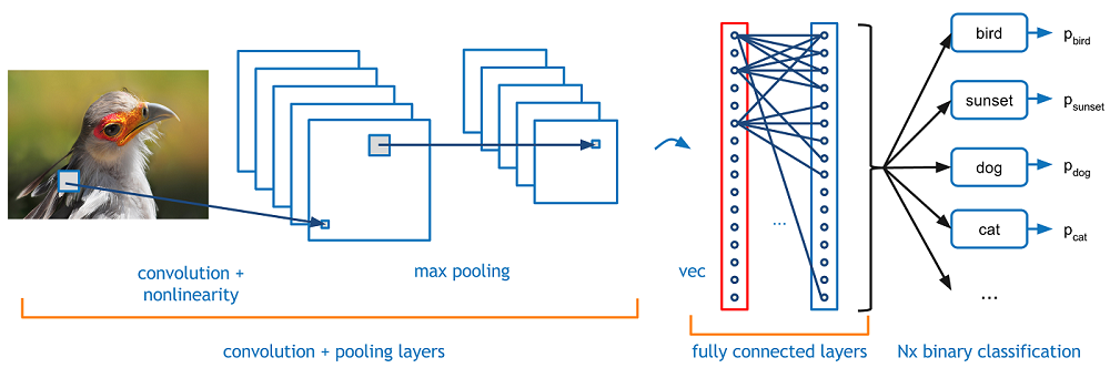
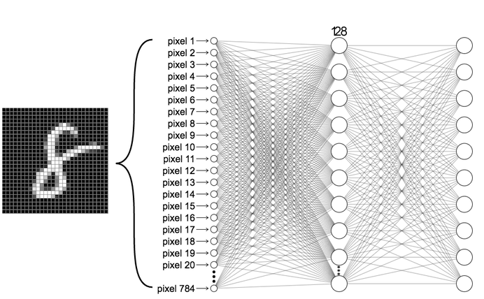
This project is a Convolutional Neural Network that will accurately predict and classify the species of an animal upon being given an image. To build this CNN, I chose to utilize two additional convolutional layers on top of VGG16, each with pooling, a flatten layer to reduce the dimensionality, a dropout layer to prevent overfitting, and finally an output layer of 10 neurons. For the convolutional layers I chose a relu activation function, since it is biologically inspired and is a general purpose function. For the last layer I chose softmax, as softmax is specialized for classification tasks. The output layer has 10 neurons to represent the 10 different classes to predict. I also gave my convolutional layers different kernel sizes so that they would hopefully pick out different features. After much internal debate, I chose the Adam optimizer. The Adam optimizer trains fast and efficiently, and combines the best features of AdaGrad and RMSprop; namely momentum and good performance on noisy datasets. My choice of loss function is categorical cross entropy. Categorical cross entropy is specialized for multi-class classifiers, making it a perfect loss function for MNIST. It also works very well with softmax, which I used.
In order to make use of the transfer learning technique, I imported VGG16 as my base model. I didn't include the top of the model, and instead made my own, featuring 3 dense layers of 4096, 512, and 10 neurons. I tried to use batch normalization, but it didn't work out and I'm not sure it would have improved my network. I also used a significant amount of dropout to prevent overfitting. To preprocess the data, I used np.dstack to reshape the images to 64, 64, 3, then used the VGG16 preprocess_input function. My learning rate was small, only 0.001. Since I have so many epochs to train, I want the learning rate to not skip over anything. I also utilized data augmentation via the ImageDataGenerator and shuffled all the data. After that, I simply wrote the results to a csv and verified accuracy. At max accuracy, I achieved 85% success.
The goal of this program was to create a basic RPC server, add several math functions, add multi-threading support, and add a key-value store (hashtable) that supports variable insertion and extraction, along with permanent storage via files. The RPC server responds to a plethora of commands, including both math, file, and hashtable functions. The RPC server accepts the connection from a client, forward it to a dispatching thread, and continue to accept connections. Meanwhile, worker threads will be 'consuming' requests from the dispatcher thread queue, and will proceed to function much like the RPC server, while also providing support for hash and additional math functions. An important aspect of this project is ensuring both the hashtable and the threads don't have synchronization issues. In order to preserve synchronicity, threads must be prevented from both receiving the same requests and entering critical regions such as the hashtable at the same time. Initially I tried mutexes and condition variables, but after a while I decided to use semaphores instead, as they are less complicated and less finicky. Upon receiving a request, the RPC server w/multi-threading will utilize the dispatch thread to enqueue the request on a queue that the worker threads have access to. The dispatch thread will continue to run in a loop infinitely, accepting any request passed to it from any connection. Semaphores are used to prevent the dispatch thread and any of the worker threads from accessing the queue at the same time. When the worker threads are alerted that there is a request waiting, one is signaled to take the request and dequeue it, processing it as quickly as possible.
The hashtable implementation used in RPC server w/multi-threading is adapted from an earlier project. It has been heavily modified to support RPC server, including editing every function, adding more functions such as load, dump, and clear, and bug-fixing. Load and dump both use fdopen, fdprintf and fscanf in order to open, scan, and print. As most hashtables are, this hashtable is an array of linked lists, with each node containing a key and value. The hash function works by rotating bits and modifying them with a hex string. Code and further explanation are available upon request.
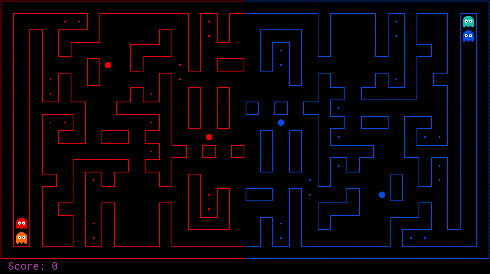
The final Pacman project I completed was in the form of a no holds-barred, tournament to the death against other students' pacman agents. I was given two ghosts that upon travelling to the enemy side of the map, become pacmen that can eat food and run from enemy ghosts. On home turf however, they merely chase enemy pacmen that make incursions upon my land. I consulted many potential strategies before settling on a strategy of 1 offense Pacman and 1 defense Pacman. Both had hand-made fine-tuned heuristics, as well as an extremely complicated expectimax search algorithm. There were a few main issues I came across. The first of which is the unpredictability of my opponents. On a macro level I did not know if my opponents were going to run double offense, offense/defense or some adaptive strategy. I had to come up with a strategy that would succeed against most of the opposition. On a micro level, I did not know how their agents would interact with ours. Would their agent chase our scared agent or would they take the opportunity to get as much food as possible? We had to look for efficient solutions to these problems as in a lot of these issues there was no clear way to always get the best outcome. Another issue we had to consider is the short computation time. What algorithm will be able to compute the best action within the given time frame? Minimax/Expectimax are search algorithms that can give us the optimal or close to optimal action, but can they execute within one second? A reflex agent is able to execute quicker, but it might not choose the optimal action given a gamestate. I had to consider and experiment with multiple algorithms to see which one would be the solution to most of my problems.
The problem of having to calculate what the enemy was going to do and act upon that turned out to be a very difficult one. Minimax/Expectimax couldn’t look very far ahead given the short computation time, and many of the other planning strategies we discussed had similar problems. In the end, I decided to not even attempt to look forward, and to instead focus on hand-built “smart” behavior that reacted to enemy behavior instead of attempting to predict enemy behavior. Following this design strategy, I decided to construct reflex agents that could make use of the now-underutilized computation time to make complicated decisions based on the gamestate. This modeled our problems in terms of choosing the best action to take out of all legal actions, based purely on the current game state. Our representation essentially framed each action as having a certain value determined by how likely it is to result in a desirable outcome. On offense, my agent should want to eat as much food as possible, and on defense, my agent should minimize the amount of food eaten by the opposition. The primary state information necessary to make a smart decision is the position of opponents and the position of food on both sides. The algorithmic choices made with the design of our reflex agents were very basic, relying mainly on iterating over opponents and food in linear time and checking the maze distance to find the closest ones. The distance to select food and opponents was used to determine the value of each action, prioritizing food on offense and prioritizing opponents on defense. In some places, the distance to the nearest opponent was used as a condition for branching to either chase or flee based on the agent type. Choosing the final action to take was simply an act of picking the highest-valued possible move based on the previous computations. Code and further explanation are available on request.
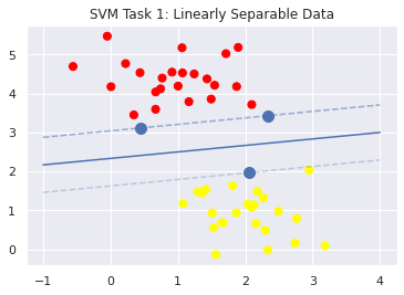
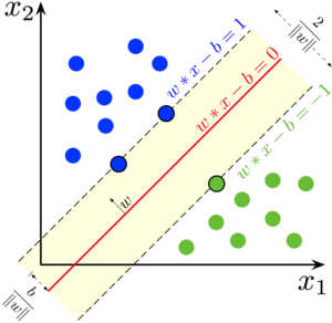
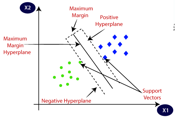
In machine learning, support-vector machines are supervised learning models with associated learning algorithms that analyze data for classification and regression analysis. In the real world, SVMs are often used for classification and separation tasks, such as email filters or the biological sciences. Given a set of training examples, each marked as belonging to one of two categories, an SVM training algorithm builds a model that assigns new examples to one category or the other, making it a non-probabilistic binary linear classifier. SVMs can also use a technique called the kernel trick wherein they implicitly map their data onto higher dimensions in order to more efficiently construct a hyperplane that cleanly divides the data. For this project, I constructed an efficient SVM using the cvxopt package. The cvxopt package allowed me to utilize the Lagrangian Dual-Formulation aspect of SVMs to make my model more efficient.
For my first task, I needed to reformulate the primal form such that it became a matrix formate and fit in the CVXOPT optimization package. I then reshaped the data, created the appropriate constants for the cvxopt solver, set tolerances, and found the appropriate weights with Strassen Matrix multiplication. Code and further explanation are available on request.
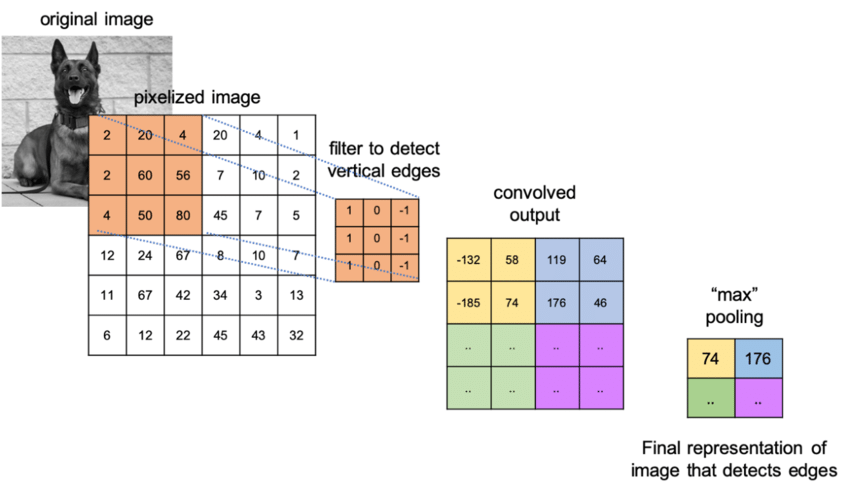
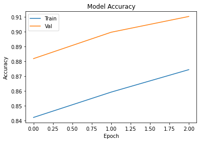
In this project I constructed a CNN by hand using the Tensorflow/Keras framework in order to recognize MNIST digits. MNIST digits are handwritten digits that are commonly used as a benchmark for visual artificial intelligence systems. Upon downloading the data, I determined its shape and form and decomposed it into arrays of 28 x 28 x 1 via numpy. I then created my Convolutional Neural Net with the Keras Functional API, hand-specifying dimensions and pooling sizes along the way. I chose to utilize two convolutional layers, each with pooling, a flatten layer to reduce the dimensionality, a dropout layer to prevent overfitting, and finally an output layer of 10 neurons. For the convolutional layers I chose a relu activation function, since it is biologically inspired and is a general purpose function. For the last layer I chose softmax, as softmax is specialized for classification tasks. The output layer has 10 neurons to represent the 10 different classes to predict. I also gave my convolutional layers different kernel sizes so that they would hopefully pick out different features. I chose adam for my optimizer, but messed around with different activation functions such as ReLu, tanh, sigmoid, and softmax to observe the different results.
At the end of it all, I managed to keep my CNN down to ~40k trainable parameters. Below is a summary of the layers of my model. Code and further explanation available upon request.
_________________________________________________________________
Layer (type) Output Shape Param #
=================================================================>
conv2d_6 (Conv2D) (None, 28, 28, 32) 320
_________________________________________________________________
max_pooling2d_6 (MaxPooling2 (None, 14, 14, 32) 0
_________________________________________________________________
conv2d_7 (Conv2D) (None, 12, 12, 64) 18496
_________________________________________________________________
max_pooling2d_7 (MaxPooling2 (None, 6, 6, 64) 0
_________________________________________________________________
flatten_3 (Flatten) (None, 2304) 0
_________________________________________________________________
dropout_3 (Dropout) (None, 2304) 0
_________________________________________________________________
dense_3 (Dense) (None, 10) 23050
=================================================================

The large amount of recorded data and statistics that are present within epidemiology make disease modeling an excellent candidate for AI-assisted generative modeling. Although the inference of how a pathogen would proliferate is a complex and high-level cognitive behavior, there exists enough neuroscience research to provide a strong tie between the organically intelligent method of solving the problem and the theoretical artificial one. Within this paper, the history and development of artificial neural networks (ANNs) are discussed, as well as their details, benefits, and limitations. A potential plan for implementation of a disease outbreak modeling network is presented, based on vector-location encodings. Additionally, natural intelligence is consulted in the theorizing and design of said model. This paper concludes with a discussion of how AI differs from the manual method, as well as potential pitfalls and advantages.
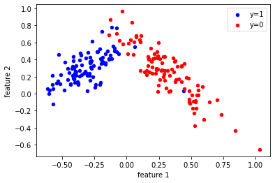
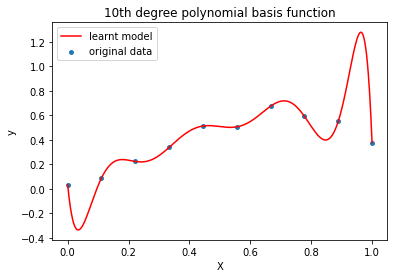
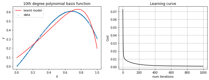
In order to get a holistic and well-rounded machine learning education, I decided to test myself against 'simpler' practices used in the past, such as linear classification and logistic regression. For many problems, these techniques are still the optimal solution, so I was happy to learn more about them! In machine learning, the goal of statistical classification is to use an object's characteristics to identify which class (or group) it belongs to. A linear classifier achieves this by making a classification decision based on the value of a linear combination of the characteristics. Logistic regression is used to obtain odds ratio in the presence of more than one explanatory variable. The procedure is quite similar to multiple linear regression, with the exception that the response variable is binomial. For linear regression I wrote a polynomial transform function in Python that transforms any data X to an nth-degree polynomial. I then wrote a linear regression program that uses gradient descent to approximate a parameter theta.
I also implemented the linear classification algorithm, or Perceptron. The Perceptron was a seminal development in the field of Artificial Intelligence, despite the fact that it cannot solve the XOR problem. I then went on to create a logistic regression program, which turned out to be significantly more complex than either of the previous exercises. I created a sigmoid function to approximate loss, a function for computing the cost/error, and a homemade gradient descent calculator in order to facilitate efficient logistic regression. Code and further explanation are available on request.

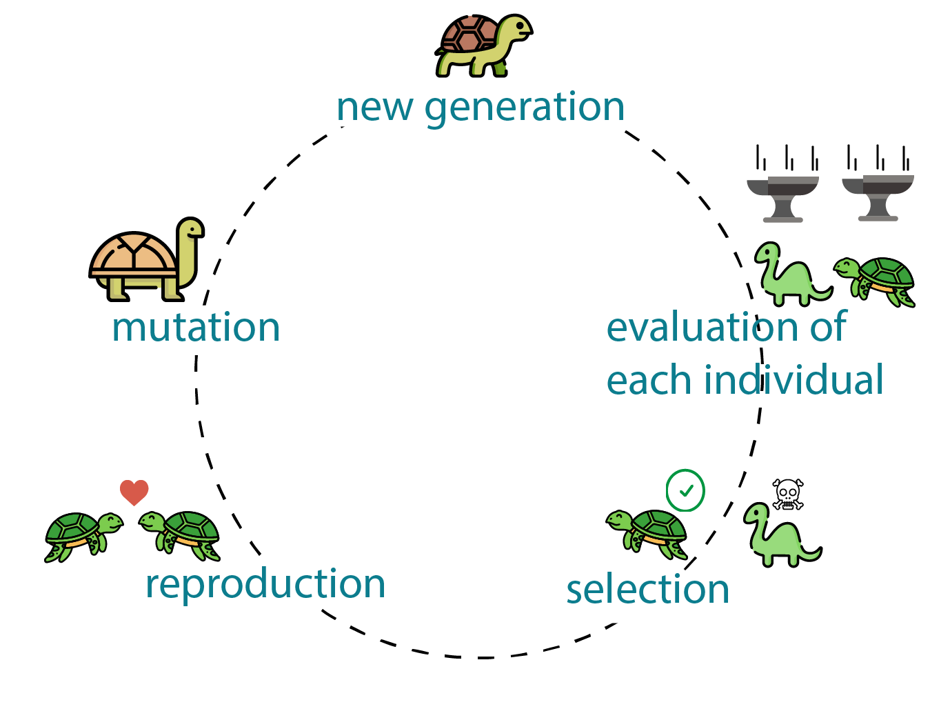
Genetic algorithms (sometimes called evolutionary algorithms) are a type of stochastic search algorithm suitable for searching large possibility spaces to find high-quality and diverse solutions. The key idea behind genetic algorithms is that two solutions might be good in some ways and bad in other ways, and combining these solutions could lead to a better solution. In genetic algorithms, we describe a problem in terms of an encoding or genome, which is necessarily problem dependent. We start with a population of individuals with distinct and diverse genomes, determine the fitness of each individual, then repeatedly select which individuals should reproduce, crossover genomes between reproducing pairs, and mutate new individuals to produce a new population. In this project I utilized two encodings. The first (Individual_Grid) treats a level as a grid of tiles represented as characters. The second (Design Elements) treats a level as a sequence of design elements like platforms, gaps, or blocks, and produces a level on the fly based on this description.
For my selection strategies, I used tournament selection and roulette selection together. The tournament method divides the population into quarters and picks the top performing genome for a given quadrant of the data set. Roulette selection attempts to make the better-performing algorithms more likely to be picked to continue on the next generation, while also eliminating any genomes with negative fitness functions. Mutate was a tricky function, which required extensive fine-tuning in order to ensure it allowed a proper amount of empty space in the level. In order to achieve an even balance of mutation, I gave each possible object a specific spawn ratio. In the case of generate_children, I simply created a child that was composed of the first half of the first parent and the second half of the second parent. We only changed the fitness function by making linearity 0.5 instead of -0.5, as it was necessary to not create worse and worse generations. To modify the fitness function for the DE encoding, I limited the amount of elements that could be present in any one level, so that every level is varied. Through natural selection and mutation, this project became able to create completely usable Mario levels on the fly, at the risk of them being a bit avant-garde. Code and further explanation available upon request.

For this project I created a rudimentary blockchain in C with no libraries. A blockchain is a growing list of records, called blocks, that are linked together using cryptography. Each block contains a cryptographic hash of the previous block, a timestamp, and transaction data (generally represented as a Merkle tree). The timestamp proves that the transaction data existed when the block was published in order to get into its hash. As blocks each contain information about the block previous to it, they form a chain, with each additional block reinforcing the ones before it. Therefore, blockchains are resistant to modification of their data because once recorded, the data in any given block cannot be altered retroactively without altering all subsequent blocks. Each block in my chain will contains three fields: data (a string that is the information stored in the block), an integer id indicating the blocks position in the chain with block 0 being the first, and a long integer value that is the hash value for the previous block in the chain. The hash value of the "previous" block in the chain is zero for the first block in the chain. The blockchain itself contains the list of Block values in the chain. My Blockchain ADT has methods append(), valid(), size(), get(), and printBlockchain() as specified in Blockchain.h. My Block ADT has methods data(), hash(), previousHash(), and printBlock() that prints the block in the format id:data, each Block id:data printed and then a newline.
Minimax deals with certainties, but its sibling, Expectimax, deals with probabilites. Since Pacman doesn't know exactly where the ghosts are going to move, he has to guess. While Minimax assumes that the adversary(the minimizer) plays optimally, the Expectimax doesn’t. This is useful for modelling environments where adversary agents are not optimal, or their actions are based on chance. My Expectimax agent ended up winning about half the time, while my Alpha-Beta agent nearly almost lost. These win percentages both increased sharply upon my devising a new and improved evaluation function that takes into account just about as many metrics as I could think of. Code and further explanation are available on request.
In this project I again created a graph module in C using the adjacency list representation. My graph module, among other things, provides the capability of running DFS, and computing the transpose of a directed graph. To find the strong components of a digraph G call DFS(𝐺). As vertices are finished, place them on a stack. When DFS is complete the stack stores the vertices ordered by decreasing finish times. Next compute the transpose 𝐺𝑇 of 𝐺. (The digraph 𝐺𝑇 is obtained by reversing the directions on all edges of 𝐺.) Finally run DFS(𝐺𝑇), but in the main loop of DFS, process vertices in order of decreasing finish times from the first call to DFS. This is accomplished by popping vertices off the stack. When the whole process is complete, the trees in the resulting DFS forest span the strong components of G.
Some of the functions I created for this project were:
Graph newGraph(int n);
void freeGraph(Graph* pG);
/* Access functions */
int getOrder(Graph G);
int getSize(Graph G);
int getParent(Graph G, int u); /* Pre: 1<=u<=n=getOrder(G) */
int getDiscover(Graph G, int u); /* Pre: 1<=u<=n=getOrder(G) */
int getFinish(Graph G, int u); /* Pre: 1<=u<=n=getOrder(G) */
/* Manipulation procedures */
void addArc(Graph G, int u, int v); /* Pre: 1<=u<=n, 1<=v<=n */
void addEdge(Graph G, int u, int v); /* Pre: 1<=u<=n, 1<=v<=n */
void DFS(Graph G, List S); /* Pre: length(S)==getOrder(G) */
/* Other Functions */
Graph transpose(Graph G);
Graph copyGraph(Graph G);
void printGraph(FILE* out , Graph G);
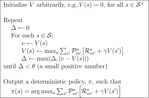
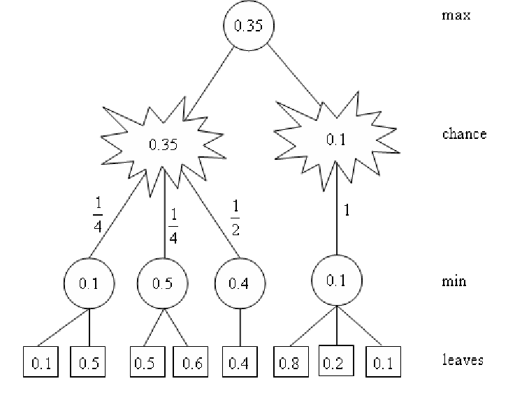
In this project, I implemented value iteration and q-learning. I tested my agents first on Gridworld (a famouse q-learning example), then applied them to a simulated robot controller (Crawler) and Pac-Man. Reinforcement learning is the training of machine learning models to make a sequence of decisions. The agent learns to achieve a goal in an uncertain, potentially complex environment. In reinforcement learning, an artificial intelligence faces a game-like situation. The computer employs trial and error to come up with a solution to the problem. To get the machine to do what the programmer wants, the artificial intelligence gets either rewards or penalties for the actions it performs. I first constructed a Value Iteration agent, an offline planner that utilizes Markov Decision Processes to find an optimal policy. Value iteration is essentially Bellman optimality paired with an update rule. Value Iteration arrives at a complete policy without ever interacting with the environment, a very different policy than q-learning.
After finishing my Value Iteration agent, I finally was able to construct a Q-Learner. Q-Learning is another name for Reinforcement Learning, a fancy name for trial and error until the computer figures stuff out. I chose to create epsilon-greedy action selection, so that my Q agent follows it's current best q-values 100% - epsilon of the time, otherwise choosing randomly. After completion of my Q-learner, I created an approximate q-learner that has the ability to learn the weights of state-features. Code and further explanation are available on request.

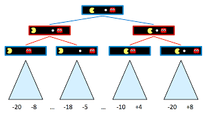
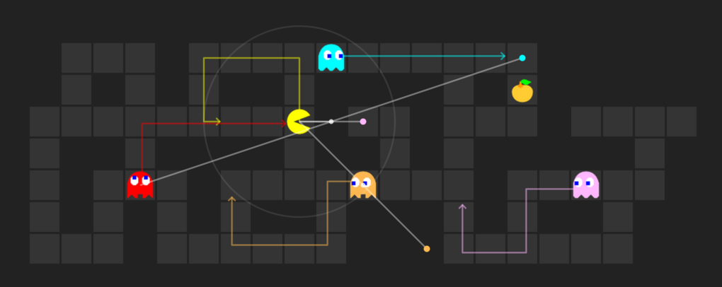
The next project to deal with Pacman involved the massive complication of multiple agents! In a game or any system, multiple actors make every action much more complex. Instead of just evaluating the static world, one must predict what one's enemies will do and attempt to counter that. Of course, they'll be doing the same thing. I first created a Reflex agent, an agent which essentially blindly wandered around seeking food and somewhat avoiding ghosts. In order to design a dynamic agent, you must be able to assign a value to each game state and pick the higher value one every time. To that end I created a host of evaluation functions that computed state-action pairs in order to find the next best move. Next up was minimax. The Minimax algorithm helps find the best move, by working backwards from the end of the game. At each step it assumes that player A is trying to maximize the chances of A winning, while on the next turn player B is trying to minimize the chances of A winning (i.e., to maximize B's own chances of winning). The minimax algorithm is excellent, but can lead to combinatorial explosion. To avoid this, you can prune parts of the game state-tree, not examining them if you already have a better (or worse) value saved in memory. This is called Alpha-Beta Pruning, and it's a tricky but worthwhile technique to use.
Minimax deals with certainties, but its sibling, Expectimax, deals with probabilites. Since Pacman doesn't know exactly where the ghosts are going to move, he has to guess. While Minimax assumes that the adversary(the minimizer) plays optimally, the Expectimax doesn’t. This is useful for modelling environments where adversary agents are not optimal, or their actions are based on chance. My Expectimax agent ended up winning about half the time, while my Alpha-Beta agent nearly almost lost. These win percentages both increased sharply upon my devising a new and improved evaluation function that takes into account just about as many metrics as I could think of. Code and further explanation are available on request.
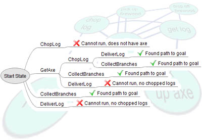
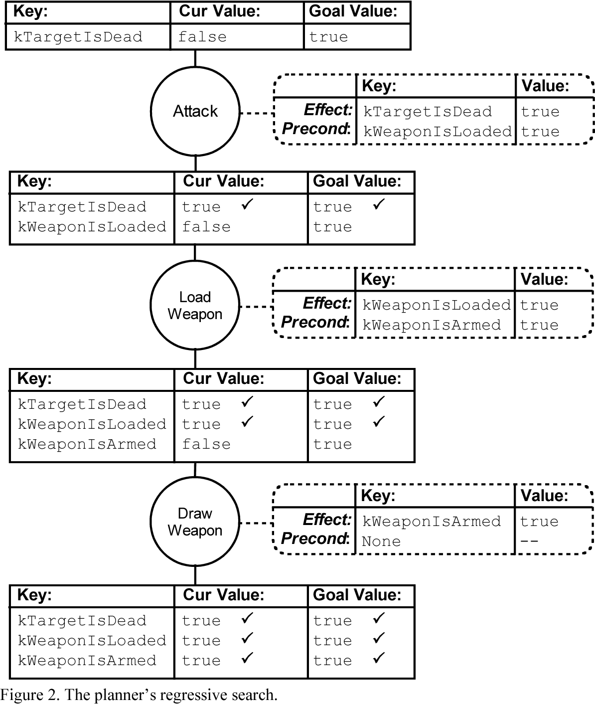
GOAP or Goal Oriented Action Planning is a powerful STRIPS (Stanford Research Institute Problem Solver) like planning architecture designed for real time control of autonomous character behavior in games. GOAP will give your agents choice and the ability to make intelligent decisions without having to maintain a complex finite state machine (FSM). In this programming project I implemented, in Python, a planner for a Minecraft-like item crafting problem. My planner is based on the A* algorithm with a unique heuristic defined for this problem. The purpose of my planner is to “craft” a set of items described by a given goal. This is achieved by taking actions which can obtain items, or which can combine items into more complex ones. In this process, some items are consumed, and others may be required but not consumed (e.g. tools). A result of an action is the generation of a new item, according to the given recipes. My goal was to define a planning problem (initial state and goal state) using these lists and to implement the A* algorithm with a heuristic.
In the interest of efficiency I constructed my solution to use backwards planning, considering first the output and reasoning from the bottom of the tree what can be done to get there. See below for an example of backwards-planning. Forward search considers the space of all possible objects that can be constructed with the initial materials, while backward search deconstructs objects, which suggests a bound to the search depth. In the backwards (or goal-regression) view, recipes apply if the requires and produces fields are true in the current state, while recipe application deletes the items in the produces field and adds the items in the consumes field to the current state. One of the many aspects I considered while designing my heuristic was redundancy. For example, if you've already crafted an iron sword but need only a wooden one, the planner can stop there. Additionally, if the planner has more than one of any required item, it doesn't need to repeatedly craft more. Code and further explanation available upon request.
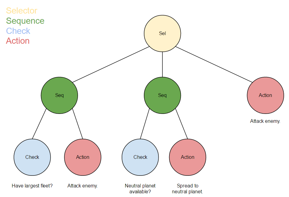
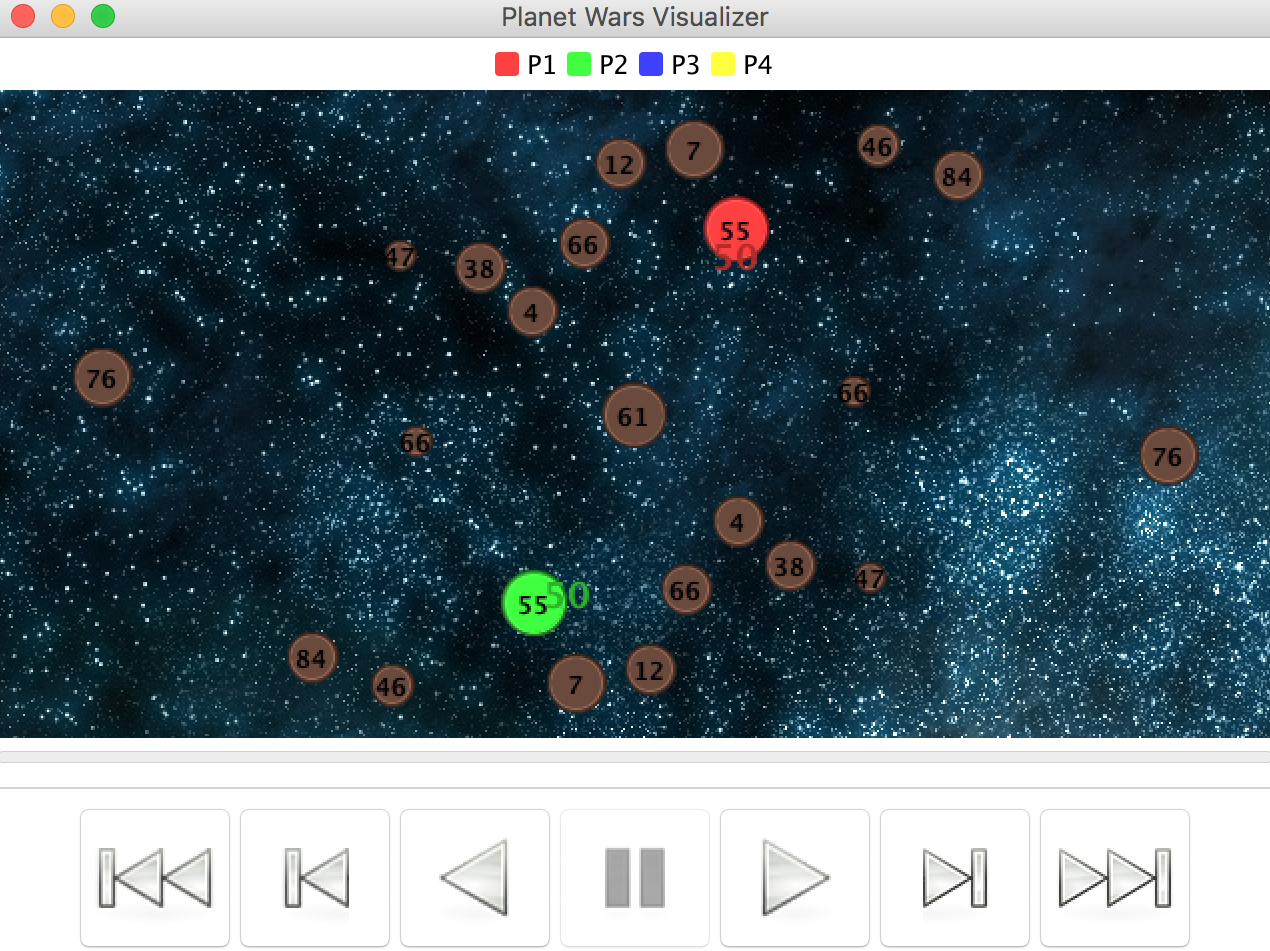
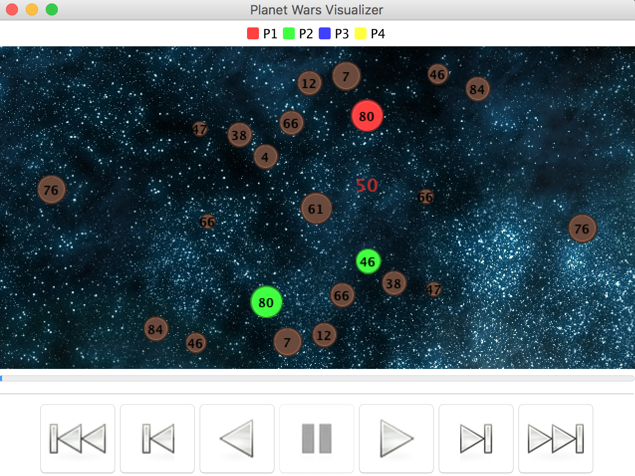
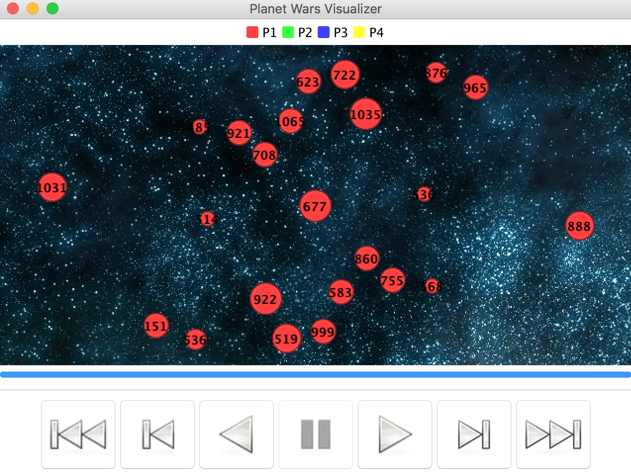
In this programming project I implemented a bot that plays Planet Wars using Behavior Trees in Python. Planet Wars is a real-time strategy game in which you have to conquer a galaxy, planet by planet. Each planet produces ships per turn, and ships can be used to take over other planets from the enemy or neutral forces (similar to Galcon). My goal wass to design a reactive bot with a single behavior tree which successfully won against a series of test bots, each representing a unique challenge and strategy. My bot was allowed to use a set of lists with important information such as a list of my planets, enemy planets, total ship production, etc. My initial strategy was to simply ignore the enemy and prioritize resource-rich planets. Specifically, the highest priority planets are big neutral planets, then cheap neutral planets, close neutral planets, and finally cheap enemy planets. The overall conquering strategy was to at first spread my fleets thin to gain resources, similar to the boardgame Risk. I also stipulated that my bot should never attack an enemy unless it's a guaranteed win, after all there is no use throwing my ships at an unconquerable enemy! The main theory used in this project was behavior tree theory.
I've provided a taste of my strategy translated to a string-tree format. Code and further explanation of the project are available upon request.
INFO:root:
Selector: High Level Ordering of Strategies
| Sequence: Offensive Strategy
| | Check: have_largest_fleet
| | Action: attack_weakest_enemy_planet
| Sequence: My Strategy
| | Check: have_largest_fleet
| | Action: attack_best_planet
| Action: attack_best_planet
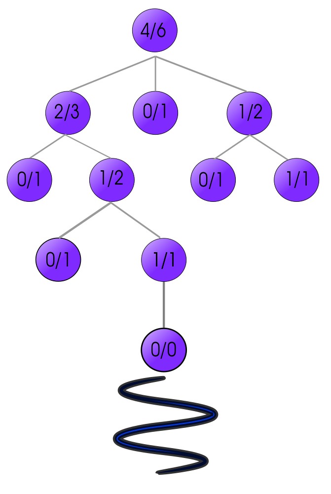
Monte Carlo Tree Search is a technique that recently been used to great success in massively complex board games such as Go or Shogi. AlphaZero/AlphaGo, the premier Go-playing software constructed by Google, makes heavy use of this fascinating technology. In my implementation of the technique, I used Ultimate Tic-Tac-Toe. Ultimate Tic-Tac-Toe is a turn-based two-player game where players have to play a grid of 9 tic-tac-toe games simultaneously in order to complete one giant row, column, or diagonal. The catch is that each on each player’s turn, they can only place a cross or circle in one square of one board; and whichever square they pick, their opponent must play on the corresponding (possibly different) board. Monte Carlo Tree Search, as you might expect from the name, uses a massive tree to search through in order to find the best possible moves to play. In the tree, every node is a game-state, a representation of all the information needed to perfectly replicate that state. More specifically, MCTS is an algorithm that figures out the best move out of a set of moves by Selecting → Expanding → Simulating → Updating the nodes in tree to find the final solution. This method is repeated until it reaches the solution and learns the policy of the game.
I first created mcts_vanilla.py, a python file that used a completely random rollout function to randomly sample possible moves that the bot could choose. Based on that, I improved the bot and added several value heuristics that helped it both prune the tree and pick better moves. A key concept in Monte Carlo Tree Search is exploitation versus exploration, or how much the algorithm should pick new, unexplored nodes to evaluate. Tweaking this formula causes large changes in performance, so that was one of the first ideas I visited in order to improve my program. The heuristic used for my first experiment reduced the exploration factor if the bot was winning the game, and increased the exploration factor when it was losing. Essentially, the logic was that if the bot has a better chance of winning currently it shouldn't waste nodes exploring. I saw greatly increased performance in the modified bot, having a higher win rate against vanilla. I also noticed it performed quite well at the start, but started to fall off eventually. Code and more explanation available upon request.
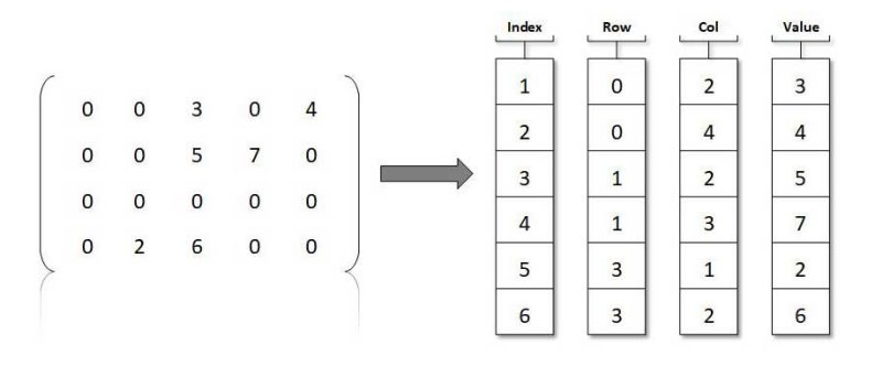
In this project I created a calculator for performing matrix operations that exploits the (expected) sparseness of it’s matrix operands. An 𝑛×𝑛 square matrix is said to be sparse if the number of non-zero entries (abbreviated NNZ) is small compared to the total number of entries, 𝑛2. As one would expect, the cost of a matrix operation depends heavily on the choice of data structure used to represent the matrix operands. There are several ways to represent a square matrix with real entries. The standard approach is to use a 2-dimensional 𝑛×𝑛 array of doubles. The advantage of this representation is that all of the above matrix operations have a straight-forward implementation using nested loops. This project used a very different representation however. Here I represented a matrix as a 1-dimensional array of Lists. This method obviously results in a substantial space savings when the Matrix is sparse. In addition, the standard matrix operations can be performed more efficiently on sparse matrices. As I saw however, the matrix operations are much more difficult to implement using this representation.
Due to the focus on efficiency in this project, the following operations were constrained to tight runtimes:
A.changeEntry(): Θ(𝑎)
A.copy(): Θ(𝑛+𝑎)
A.scalarMult(x): Θ(𝑛+𝑎)
A.transpose(): Θ(𝑛+𝑎)
A.add(B): Θ(𝑛+𝑎+𝑏)
A.sub(B): Θ(𝑛+𝑎+𝑏)
A.mult(B): Θ(𝑛2+𝑎⋅𝑏)

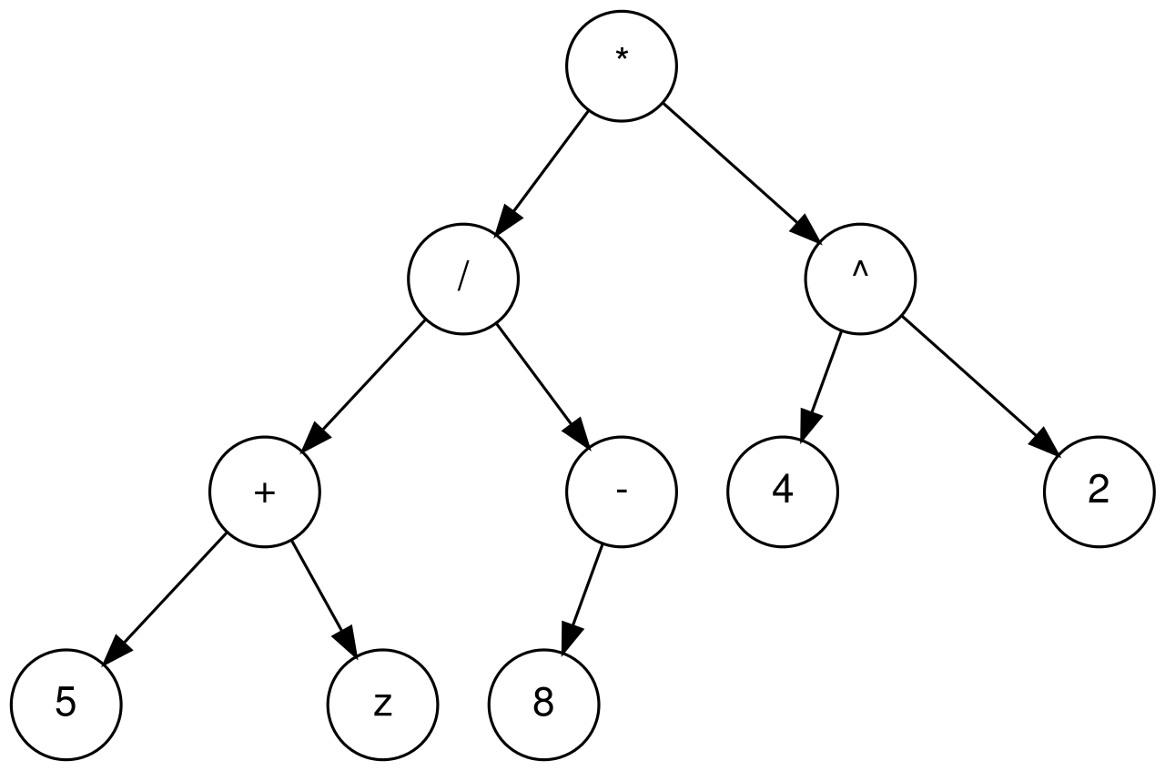
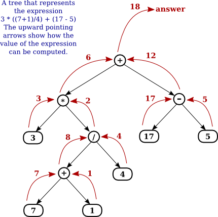
An Expression tree is a binary tree in which each internal node corresponds to operator and each leaf node corresponds to operand. To build an expression tree I accepted input in post-fix notation, also known as Reverse Polish Notation (RPN) which scientific calculators continue to use. The stack implementation I created is a stack of void * pointers which means that the stack can hold references to any kind of object. It is not bound to the kind of items are stored in the stack. There is no type checking of items added to the stack. The programmer overrides the compiler’s type checking system and casts the pointer to the right type. The final PostFixCalculator program builds the Expression Tree then prints the inorder traversal with parentheses (including each integer argument to make things easier), then prints the evaluation of the expression. The calculator will accept only integer values and the arithmetic operators.
The algorithm I followed for this project was:
Loop through input expression and do the following for every token (a set of non-whitespace characters)
1) If token is operand push that into stack
2) If token is operator pop two nodes from stack make them its child and push the current node again.
At the end the only element of stack will be the root of the expression tree.
In this project, I wrote a Java program that uses recursion to find all solutions to the n-Queens problem, for 1≤𝑛≤15. The Eight Queens puzzle is to find a placement of 8 queens on an otherwise empty 8×8 chessboard in such a way that no two queens confront each other. Solutions are encoded as an 𝑛-tuple where the 𝑖th element is the column number of the queen residing in row 𝑖. My program represented an 𝑛×𝑛 chessboard by a 2-dimensional int array of size (𝑛+1)×(𝑛+1). The extra row and column are there so row and column numbers in the array correspond directly with row and column numbers on the chessboard. Specifically, if the array is called B, then B[i][j] corresponds to the square in row i, column j of the chessboard. The program operates in two modes: normal and verbose (which is indicated by the command line option "-v"). In normal mode, the program prints only the number of solutions to n-Queens. In verbose mode, all solutions to n-Queens will be printed in the order they are found by the algorithm, and in a format described below, followed by the number of such solutions.
I have provided high-level pseudocode for my solution below:
1. if 𝑖>𝑛 (a queen was placed on row 𝑛, and hence a solution was found)
2. if we are in verbose mode
3. print that solution
4. return 1
5. else
6. for each square on row 𝑖
7. if that square is safe
8. place a queen on that square
9. recur on row (𝑖+1), then add the returned value to an accumulating sum
10. remove the queen from that square
11. return the accumulated sum

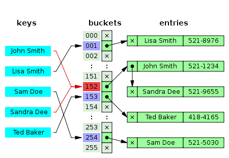
A hash table is simply an array that is used to store data associated with a set of keys. In my Dictionary ADT I store a set of (key, value) pairs where keys and values are C strings (i.e. null '\0'terminated char arrays). If the keys all happen to be in the range 0 to N - 1, and Ni s not too large, one can simply allocate an array of length N, and store the value vin array index k. This arrangement is called a direct-address table. There is of course one problem: two keys may hash to the same slot. We call this situation a collision. I dealt with collisions by chaining nodes onto each other in a linked list ADT. At that point the only question left was what to choose as my hash function. A good hash function should satisfy (at least approximately) the assumption of simple uniform hashing: each key is equally likely to hash to any of the mslots, independently of the slot to which any other key has hashed. For this reason and because I had no reason not to, I chose SuperFastHash. Code and further explanation are available upon further request.

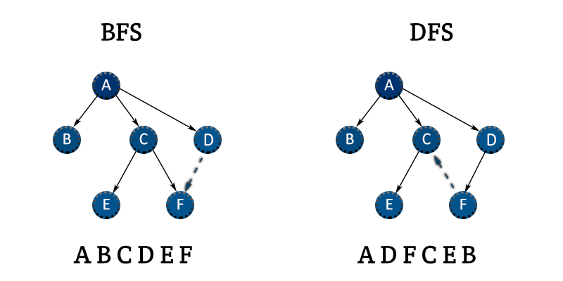
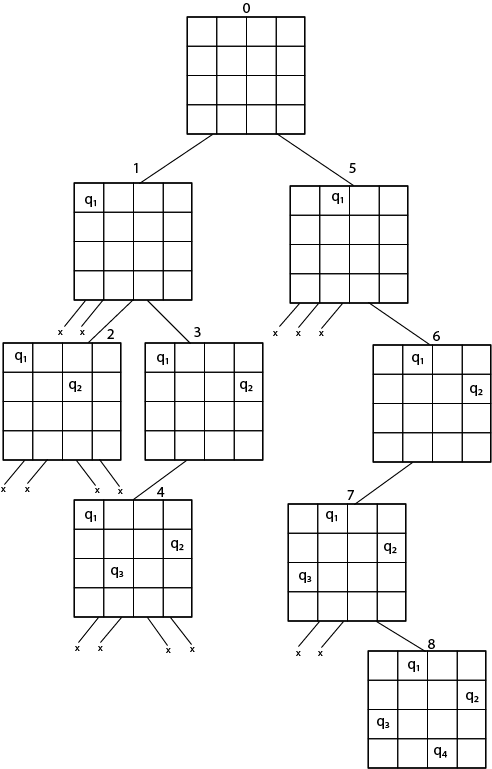
This was a relatively simple project that I completed to familiarize myself with the Pacman environment I was going to be using for the next few projects. In order to demonstrate basic competency in both Python and AI concepts, I implemented A*, Dijkstra's, BFS, DFS, and Uniform Cost Search for Pacman to find every food dot in his maze. To do this I utilized several data structures, including but not limited to doubly linked lists, queues, priority queues, stacks, lists, sets, and more. For A* specifically I used the fringe idea, a slightly different formulation of the classic A* algorithm. Code and further explanation are available on request.
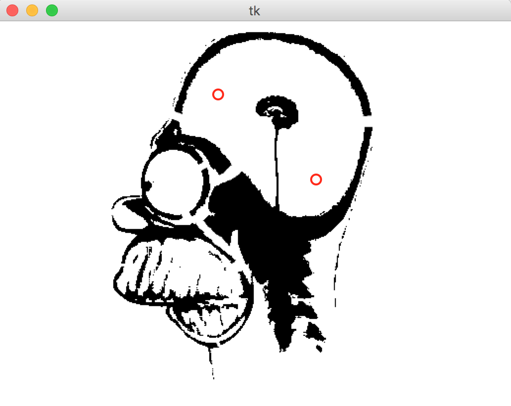
In this programming project I implemented in Python a bidirectional A* search algorithm to solve the problem of finding paths in navmeshes created from user-provided images. The input parameter is a navmesh and the output is an image showing the path from a source and destination. Both the source and the destination are defined interactively through a python program. A navmesh is an abstract data structure used in AI and specifically pathing that highlights travelable areas of a map. In this case, the navmesh was an image of an X-ray of Homer Simpson that was broken down into many discrete rectangles of various shapes and sizes. My first step in the implementation was to identify the source and destination boxes and their locations within the overall image by searching the adjacency list of boxes given to me. I then implemented an inefficient but complete version of Dijkstra's Search, just to make sure that the destination box was actually reachable from the initial box. I then modified my search to be comprised of a series of line segments, originating from the center of the initial box and traveling to the center of the destination box. These line segments intersect the boundaries of boxes at the point where the corner of a neighboring box touches the first box.
For a more intuitive explanation, please view the image below. I then changed my initial implementation of Dijkstra's Search into a bidirectional A* search that utilized a queue. image. Utilizing a little bit of mind-bending geometry, I repeatedly find the euclidean distance between two points, as well as find the closest point on a line segment in relation to a given point. Without giving too much away, I was able to create an optimal search and pathing function for any given rectangularly-segmented navmesh, a non-trivial problem. Additionally, if there is no path possible, that is reported back to the user, as well as a variety of other edge cases. Code is available upon request.

This project introduced me to the MIPS ISA using MARS, a Missouri State Assembly language designed for educational purposes. I created a program that outputted ASCII triangles of various sizes depending on user input. For example, if the user inputted the number 7, the program created a looping diagonal triangle with sides of 7 slashes or '\'s. Specifically, this program prompted the user for two integers: the length of one of the legs of a triangle and the number of triangles to print. Next, the program printed triangles to the console based on the user input. After printing the specified numberof triangles, the program quits. I used at maximum 10 registers for this project, which severely limited the amount of memory I had access to. Luckily, it helped teach me constraints in close to the metal programming. This was also my first experience with loops in assembly, an aspect of OOP that is extremely important. Using too many branches or loops is deleterious in Assembly, as you start getting closer and closer to spaghettification. Code is available on request.